Trying out gganimate

Load R packages

library(splatter)   # simulate scRNA-seq data
library(scater)     # use the logNormCounts() function from here
library(Seurat)     # manipulating the scRNA-seq data
library(tidyverse)  # data wrangling
library(gganimate)  # fancy plots

Simulate data

I’ll simulate 400 cells transitioning along a continuous differentiation trajectory with four paths, each cell having an equal probability of belonging to each. I’ve become more familiar with the structure of Seurat objects for handling single cell data, so along the way we’ll convert the SingleCellExperiment object to a Seurat object before identifying variable features and running PCA.

# Simulate data
params.groups <- newSplatParams(batchCells = 400,
                                nGenes = 800)
sim1 <- splatSimulatePaths(params.groups,
                           path.nSteps = 10,
                           group.prob = rep(0.25, 4),
                           de.prob = 0.5,
                           de.facLoc = 0.2,
                           path.from = c(0, 1, 2, 3)) %>%
  logNormCounts() %>%
  as.Seurat() %>%
  FindVariableFeatures() %>%
  ScaleData() %>%
  RunPCA()

Peek at the metadata:

head(sim1@meta.data)
##        Cell  Batch Group ExpLibSize Step sizeFactor
## Cell1 Cell1 Batch1 Path4   74225.82    2  1.2209645
## Cell2 Cell2 Batch1 Path3   63802.26    6  1.0352153
## Cell3 Cell3 Batch1 Path2   76739.30    2  1.2754246
## Cell4 Cell4 Batch1 Path3   46640.71    8  0.7478661
## Cell5 Cell5 Batch1 Path3   58112.13    6  0.9680266
## Cell6 Cell6 Batch1 Path3   57435.94    6  0.9348244

Splatter approximates a continuous trajectory by simulating a series of steps between groups. We specified four groups and 10 steps per group. Let’s add a new variable to approximate time:

# Get group info as numeric (integer between 1-4) then multiply by ten
sim1$Time <- as.numeric(str_remove_all(sim1$Group, "Path"))*10 
#  Add step info (integer between 1-10)
sim1$Time <- sim1$Time + sim1$Step 
# start from zero not ten
sim1$Time <- sim1$Time - 10 

Static plot

Create some static PCA plots highlighting the Time variable we created and the paths and steps.

# Plot group (paths), steps and our new Time variable using two of Seurat's built in 
# plot functions; DimPlot() and Featureplot()
DimPlot(sim1, group.by = "Group")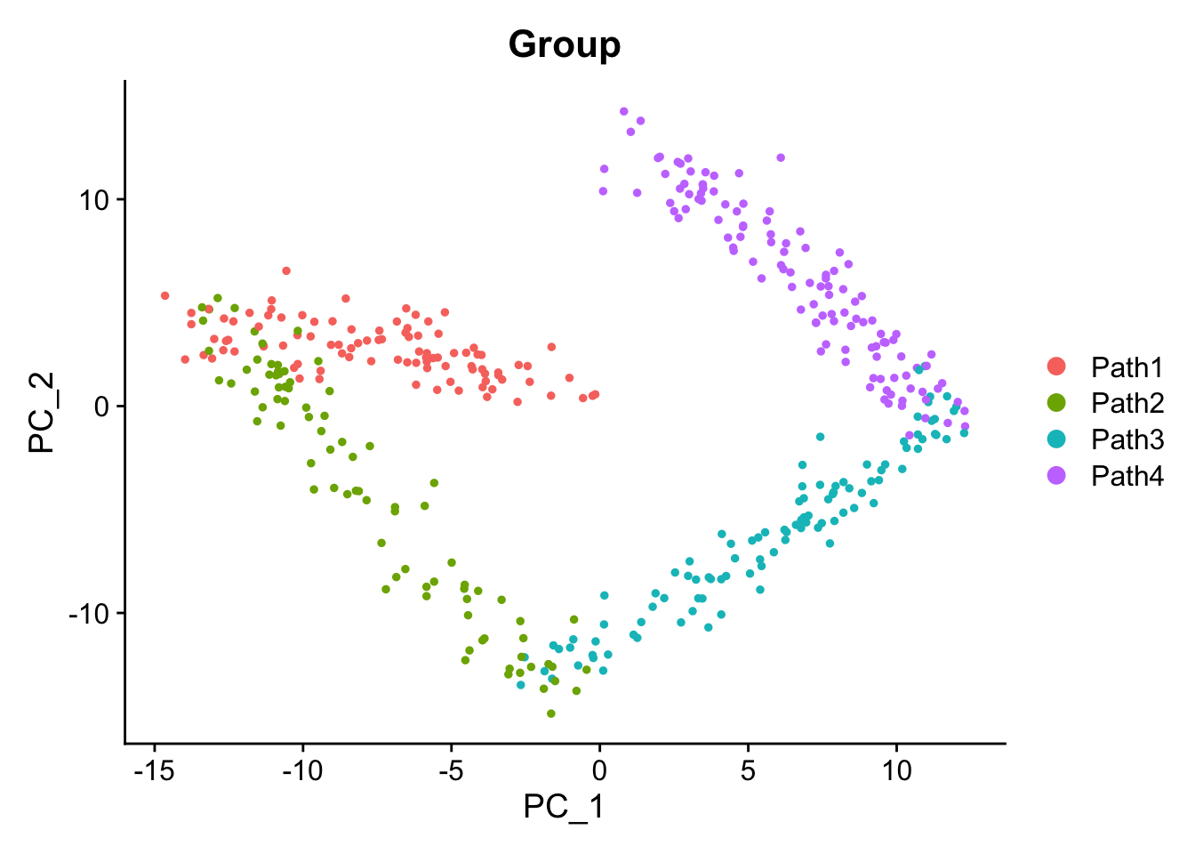 

FeaturePlot(sim1, "Step") + scale_color_viridis_c()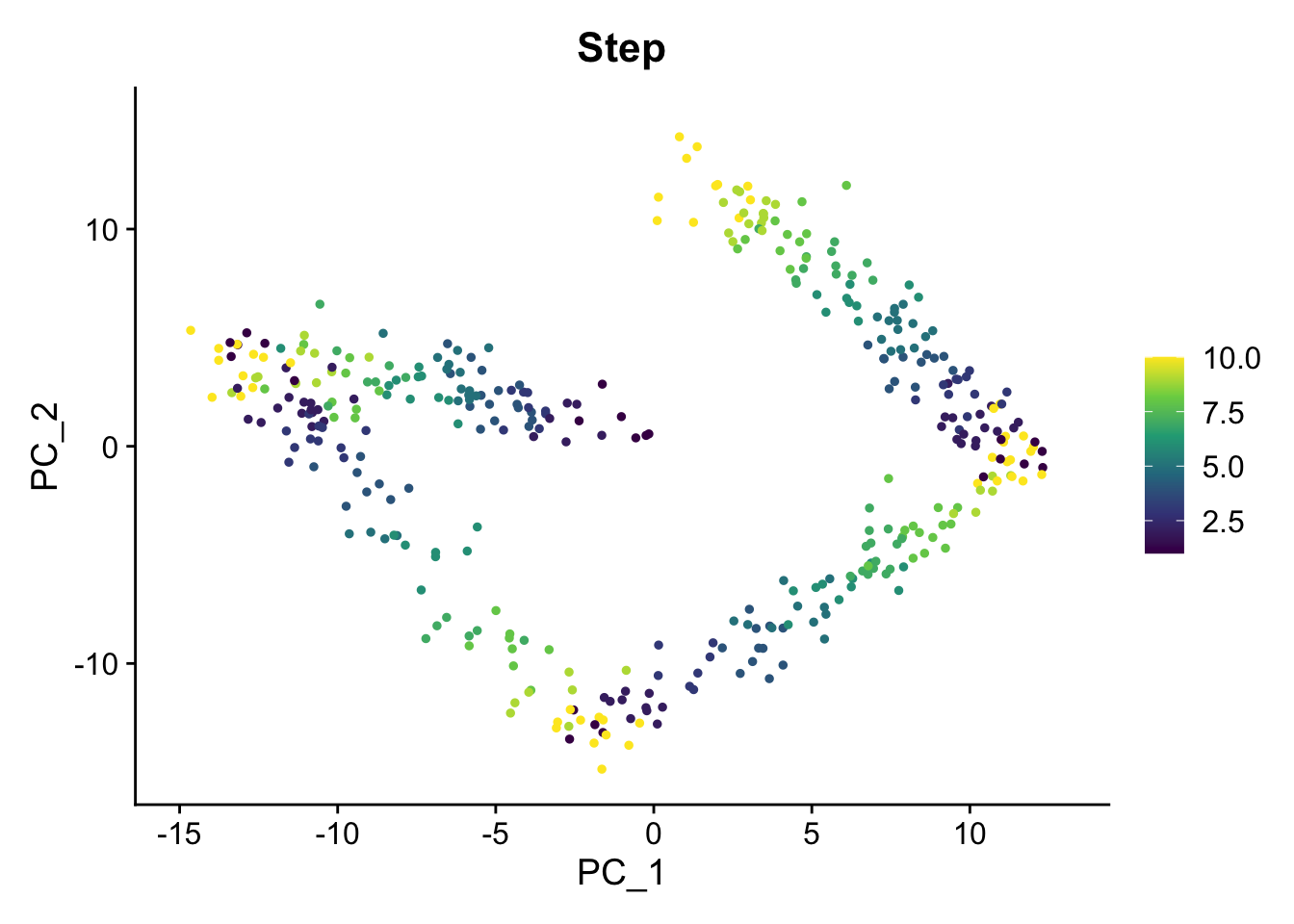

FeaturePlot(sim1, "Time") + scale_color_viridis_c()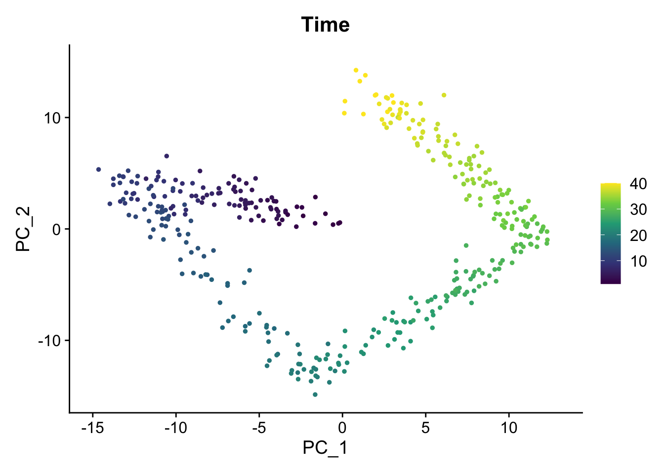

Dynamic plot

Now we’ll use the Time variable to animate the plot. We use the shadow_mark argument to keep track of the path of the cells so that they don’t just disappear from frame to frame.

# Pull data for plotting
plt.data <- cbind(sim1@meta.data,
                  Embeddings(sim1)[, 1:2])

# Create a static plot
p <- ggplot(plt.data, aes(x = PC_1, y = PC_2, col = Time)) +
  geom_point() +
  scale_colour_viridis_c()

# Add some animation
anim <- p +
  transition_states(Time,
                    transition_length = 2,
                    state_length = 1) +
  ggtitle('Time: {closest_state}') +
  shadow_mark(alpha = 0.5, size = 0.7)

animate(anim)

I think the colour in the static plot does the job of conveying the trajectory of the cells through time and adding animation doesn’t contribute much. But it was good to try out gganimate anyway and discover that the grammar makes it easy to add animation to normal ggplots. Now I’ve finally tried it out I can keep an eye out for future datasets where it might come in handy. Also first post!!! 🎉 🎉